Gaussian Splatting viewer in OpenGL, using LOVR
Martino Trapanotto / November 2024 (5094 Words, 29 Minutes)
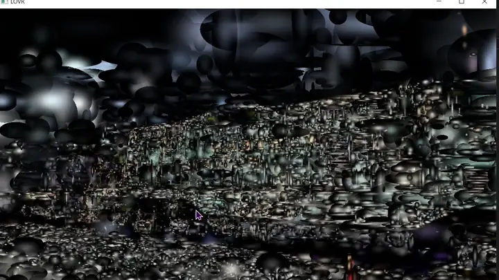
A few months back, I learned about Gaussian splatting while finishing work on my thesis, and it got me quite curious. For obvious reasons I couldn’t focus on it too much, but the desire to explore the topic remained.
After my graduation in July, I finally had some spare time, and to better immerse myself in the topic I decided to implement a relatively simple renderer for gaussian splatting scenes. This took a couple of months, between understating the logic, finding an OpenGL implementation to study and fixing a lot of bugs, differences and more.
But now, I have my own personal custom GMO-free unique organic OpenGL-based range-free open source Gaussian Splatter!
Starting out
The first step is always the same: watching YouTube videos to coax myself in a false sense of self-confidence. If it can be vaguely explained in a few minutes in a video, how hard could it ever be?
After that, I collected some basics: the original paper, a simple OpenGL implementation, a topic review and some internet tutorials.
This deeper research phase surfaced a bunch of additional questions I wanted to answer to understand the context this tech exists in, and I’ll summarize the answers here for anyone who also had no idea how we got here:
Nomenclature and context
- Novel View Synthesis is the general task of being able to see a scene from a view that was not originally collected, like watching a movie from a new angle. It’s the main objective of 3D Gaussian Splatting (3DGS).
- NeRFs or Neural Radiance Fields are the previous step in the evolution of View Synthesis before 3DGS, using a neural network to learn the radiance field of the scene. They’re quite good, but slower in training and rendering, opaque to studying them and modifying them and generally share black box issues with other NNs.1
- Radiance Field is the mathematical representation of a scene’s appearance in 3D. It’s a mapping, that maps positions and direction to RGBa values. This is usually combined with Volumetric Ray Marching.
- Volumetric Ray Marching is a technique to render a non-opaque volume, by defining a ray and sampling colors and opacities along the ray.
- SLAM and SfM (Simultaneous Location And Mapping and Structure from Motion respectively) are basically both the task of constructing a 3D mapping of a scene, usually as point clouds, given a video/collection of views. SfM is the name used in Computer vision tasks, while SLAM is more commonly used in robotics.
In the case of NeRFs, the network is trained and to render a view, you give it a pose, then you use Volumetric Ray Marching, sampling using the NeRF along the view rays. This gives you the color and opacity in the volume you’re looking at. After combining them you have your novel view. Cool, but quite slow and hard to optimize.
What Gaussian splatting introduces
The original paper introduces a bunch of things together, including the usage of 3D Gaussians, how to render them to a 2D image efficiently and how to construct a scene out of gaussians by starting from SLAM data.
The very high level concept is that these semi transparent gaussians can be initialized from the point cloud data, then using the known views of the scene they can be refined, changing color, splitting and multiplying and culling, until we have a high quality reconstruction of the scene.
These introduce a bunch of advantages on NeRFS:
- they’re faster to render and train, by far
- they’re higher quality
- their structure is explicit, you can easily modify a scene without retraining, even by hand
Here you’ll probably have a crystal clear picture of how limited my art training is, but I like to liken the gaussians to a 3D version of a brush stroke: the painter (the gradient descent) perceives a view and adds layers of colors and strikes (the gaussians) to reconstruct what they perceive. The strokes layer onto each other, combining and blending into creating the illusion of a complex image, from individually simple elements.
Actually building
Now that we have some background, let’s move to rendering.
As mentioned, I borrowed quite heavily from the Gaussian Splatting Viewer by Li Ma. I chose this as it was a relatively simple Python+OpenGL implementation I could use as a reference, and didn’t seem to do much more than rendering.
I’m also not writing it in C++ and OpenGL from scratch, I’m using the 3D/VR framework LOVR to instead use Lua and OpenGL. This allows me to avoid thinking about memory management, file access, compiling and distribution on various platforms and allows me to more easily use OpenGL interactively. LOVR is a framework I’ve grown to really appreciate in its flexibility and simplicity, alongside performance and openness, and you might have seen it in other posts here.
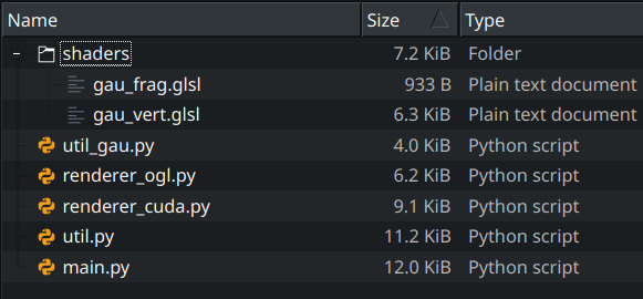
Getting back at the reference viewer, we can look through the source and understand which files are of interest (I already removed caches, requirements, licenses and more):
Of the remaining:
renderer_cuda.pyshould be for the CUDA, backend, and I don’t know much about CUDA, nor can I run it on this machinemain.pymostly manages inputs, GUI, loading backends and such, but nothing much about exactly how the rendering worksutil_gau.pycontains mostly data loading and processing, a dataclass for the gaussians and the demo scene. Nice for later, but not too importantutil.pyhas a lot more for us, with a bunch of OpenGL wrappers and the properties and functions of the virtual camera, along some inputs
The real meat is in render_ogl.py, where we find the shader compilation stage, data passing between CPU and GPU, details on the drawn objects and on the OpenGL calls and settings.
Also, highly important are the OpenGL shaders in the shaders folder (what a deduction!), which tell the GPU how to process the data passed to it by Python.
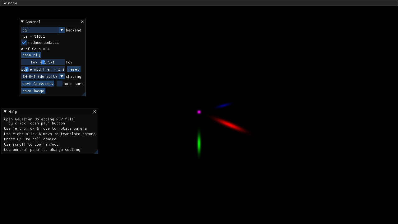
So as a first objective I settled on recreating the demo scene that the Viewer opens to, with only 4 gaussians to demonstrate the tech.
Instances and Quads
To summarize a few weeks of trials and errors (mostly errors), in render_ogl.py we can see these important lines:
class OpenGLRenderer(GaussianRenderBase):
    def __init__(self, w, h):
        ...
        self.program = util.load_shaders('shaders/gau_vert.glsl', 'shaders/gau_frag.glsl')

        # Vertex data for a quad
        self.quad_v = np.array([
            -1,  1,
            1,  1,
            1, -1,
            -1, -1
        ], dtype=np.float32).reshape(4, 2)
        self.quad_f = np.array([
            0, 1, 2,
            0, 2, 3
        ], dtype=np.uint32).reshape(2, 3)

        # load quad geometry
        vao, buffer_id = util.set_attributes(self.program, ["position"], [self.quad_v])
        util.set_faces_tovao(vao, self.quad_f)
        self.vao = vao
        ...
        gl.glBlendFunc(gl.GL_SRC_ALPHA, gl.GL_ONE_MINUS_SRC_ALPHA)
        ...

    def draw(self):
        '''I think calls the rendering pipeline'''
        gl.glUseProgram(self.program)
        gl.glBindVertexArray(self.vao)
        num_gau = len(self.gaussians)
        gl.glDrawElementsInstanced(gl.GL_TRIANGLES, len(self.quad_f.reshape(-1)), gl.GL_UNSIGNED_INT, None, num_gau)
Here there are two key parts:
gl.glDrawElementsInstanced, which tells us it’s using instanced renderingquad_fandquand_v, which tell us what is being instanced. These are stored in theself.vao
Instanced Rendering is a common technique for rendering a huge number of identical models, with some modifications done to them. Think grass or particles or maybe crowds, where you might want to add noise or colored effects, but don’t need excessive control and instead want better performance.
Instead of producing a call to the GPU for each object, these are batched together in a single huge call, and any modifications that the individual instance might need is handled by a custom shader. This removed a lot of wasted time, reduces memory consumption and allows the CPU and GPU to better work independently.
So if we read on the pyOpenGL docs about how the call works, we learn that we are calling num_gau instances to be drawn, and that the self.vao contains info on what is being drawn.
So how are we using these vertices again?
Vertices
We can look int the first of the two shaders, gau_vert.glsl.
As the filename implies this is a Vertex Shader, so it processes vertex data.
Inside we can find some important pieces of information:
void main()
{
	// Gaussian number
	int boxid = gi[gl_InstanceID];
	// Number of elemenets encoding the splat
	int total_dim = 3 + 4 + 3 + 1 + sh_dim;
	// initial offset to reach the ith element
	int start = boxid * total_dim;
	// Get position and associated matrices
	vec4 g_pos = vec4(get_vec3(start + POS_IDX), 1.f);
    vec4 g_pos_view = view_matrix * g_pos;
    vec4 g_pos_screen = projection_matrix * g_pos_view;
	g_pos_screen.xyz = g_pos_screen.xyz / g_pos_screen.w;
    g_pos_screen.w = 1.f;
    // Load rotation scale and opcatity data
	vec4 g_rot = get_vec4(start + ROT_IDX);
	vec3 g_scale = get_vec3(start + SCALE_IDX);
	float g_opacity = g_data[start + OPACITY_IDX];
    ...
Here, gl_InstanceID defines the instance itself, so which gaussian we are drawing.
total_dim and start and those *_IDX are there to access the attributes of each gaussian through the get_vec functions, because here all the data is stored in a single larger data buffer:
layout (std430, binding=0) buffer gaussian_data {
	float g_data[];
	// compact version of following data
	// vec3 g_pos[];
	// vec4 g_rot[];
	// vec3 g_scale[];
	// float g_opacity[];
	// vec3 g_sh[];
};
...
main(){
...
Why? I’m not sure, maybe it’s more memory efficient or faster, or they found it easier to work with. I find it confusing.
Here we also can check what data the gaussians need exactly:
vec3Positionvec4Rotationvec3ScalefloatOpacityvec3Spherical Harmonics
This data is loaded in the buffer in render_ogl.py via update_gaussian_data. To learn more about Spherical Harmonics, I have another blog post.
From here we see that it’s either loaded from a Ply file or from the naive demo we discussed earlier.
Next step: using this data
...
mat3 cov3d = computeCov3D(g_scale * scale_modifier, g_rot);
vec2 wh = 2 * hfovxy_focal.xy * hfovxy_focal.z;
vec3 cov2d = computeCov2D(g_pos_view,
                            hfovxy_focal.z,
                            hfovxy_focal.z,
                            hfovxy_focal.x,
                            hfovxy_focal.y,
                            cov3d,
                            view_matrix);

// Invert covariance (EWA algorithm)
float det = (cov2d.x * cov2d.z - cov2d.y * cov2d.y);
if (det == 0.0f)
    gl_Position = vec4(0.f, 0.f, 0.f, 0.f);

float det_inv = 1.f / det;
conic = vec3(cov2d.z * det_inv, -cov2d.y * det_inv, cov2d.x * det_inv);

vec2 quadwh_scr = vec2(3.f * sqrt(cov2d.x), 3.f * sqrt(cov2d.z));  // screen space half quad height and width
vec2 quadwh_ndc = quadwh_scr / wh * 2;  // in ndc space
g_pos_screen.xy = g_pos_screen.xy + position * quadwh_ndc;
coordxy = position * quadwh_scr;
...
It’s not so obvious, is it?
computeCov3D computes the 3D Covariance matrix of the gaussians.
If you’re following from home with the original paper on the side, we’re in section 4, and this function produces the matrix that represent the Gaussian we’re drawing.
I’m pretty sure this can be done ahead of time instead of at each frame, as it depends only on the data loaded from disk, and could be computed after loading. Might be a first optimization for later.
hfovxy_focal and hw store info about the virtual camera, basically only window resolution. These are components of
computeCov2D projects the gaussina in 2D based on position and camera effects, by approximationg perspecive effects. The math comes from a 2001 paper, and more matematically here we create and matrices and combine them with to produce , which is also filtered to only X, Y and XY covariances.
det is the determinant of the covariance matrix, allowing us to check if the gaussian is completely invisible from this view with (det == 0.0f) and to compute the conic, which just stores the covariance in a normalized format for later usage.
quadwh_scr and quadwh_ndc eluded me for weeks, until I understood that they represent the size of the quad: one in pixels and one in normalized screen space. I think the 3 here is to have a quad 3 times the variance of the gaussian, so covering 99% of it.

From here the rest of the shader is relatively clear:
g_pos_screen.xy = g_pos_screen.xy + position * quadwh_ndc;
coordxy = position * quadwh_scr;
gl_Position = g_pos_screen;

alpha = g_opacity;

if (render_mod == -1)
{
    float depth = -g_pos_view.z;
    depth = depth < 0.05 ? 1 : depth;
    depth = 1 / depth;
    color = vec3(depth, depth, depth);
    return;
}

// Covert SH to color
int sh_start = start + SH_IDX;
...
color = SH_C0 * get_vec3(sh_start);
In OpenGL, gl_Position stores the position of the vertex we’re working on, so by overriding it here we manipulate the corners of the quad, and thus control it’s size to match the gaussian.
position stores the local coordinates of the object being drawn, so the corner of the quad in question.
Only of note, is that I’m not interested in delving deeper in the spherical harmonics this time. I wrote an entire blogpost on them before, and I’ll only be using the 0th order for flat coloring.
Fragments
The fragment shader gau_frag.glsl is a lot less busy:
void main()
{
    ...
    float power = -0.5f * (conic.x * coordxy.x * coordxy.x + conic.z * coordxy.y * coordxy.y) - conic.y * coordxy.x * coordxy.y;
    if (power > 0.f)
        discard;
    float opacity = min(0.99f, alpha * exp(power));
    if (opacity < 1.f / 255.f)
        discard;
    FragColor = vec4(color, opacity);
...
}
Here we compute power, which produces the bellcurve effect of the gaussian, and add it to the alpha of the pixel, completing the rendering pipeline.
Now we can load the bigger scene from disk. This is boring and I’ll gloss over it. I had to convert to ASCII PLY to parse it quickly in Lua, and then load the data in buffers. Not interesting, just ugly and fragile.
So, are we done?
Transparency
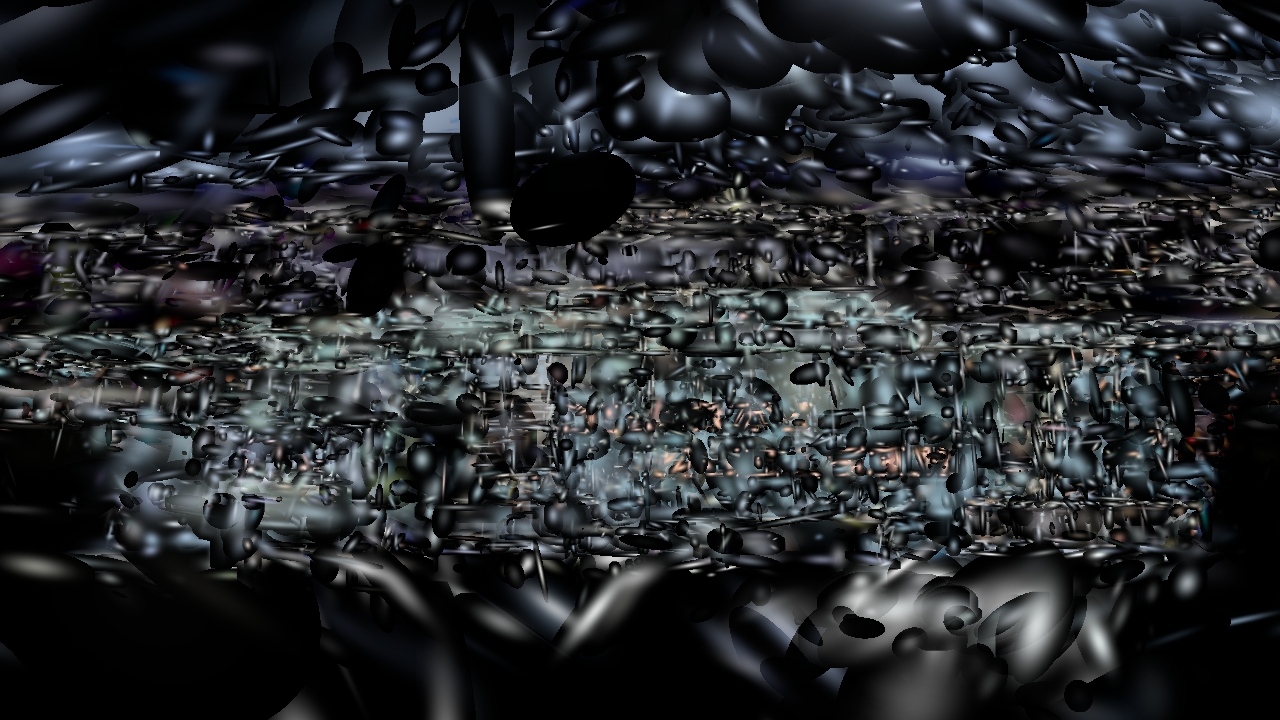
We forgot that transparency is not a trivial task in computer graphics.
In 3D graphics we generally produce transparency via Alpha compositing, also called Blending, where we layer the colors onto each other. This requires the rendering to be done in order, back to front or front to back depending on the formula used.
Here, and are the input RGB colors, with the output, and the s represent their opacity. This operator, called “Over” is order dependent, so we need to sort the gaussians and pass this info to the GPU.
This might sound impossible with a GPU, as it’s supposed to work in parallel, processing and shading multiple elements independently. But that’s not entirely true, and we can actually fix this.
This is done by quite literally computing the draw order in CPU and passing it to the GPU as a buffer.
It appears in the vertex shader only, and it’s used to choose at which gaussian to start reading:
...
layout (std430, binding=1) buffer gaussian_order {
	int gi[];
};
...
void main()
{
	int boxid = gi[gl_InstanceID];
...
Its contents are managed by render_ogl.py:
...
    def sort_and_update(self, camera: util.Camera):
        '''Resort rendered gaussians based on view position'''
        index = _sort_gaussian(self.gaussians, camera.get_view_matrix())
        self.index_bufferid = util.set_storage_buffer_data(self.program, "gi", index, bind_idx=1,buffer_id=self.index_bufferid)
        return
The sorting is done by simply taking the view matrix, computing the relative position of the gaussians and ordering by Z value. Then we store the indexes and pass them to the GPU.
By telling the GPU to pick from these based on the Instance Index, we know that the drawing will follow the same ordering, so we can draw back to front.
And with that, we have a decent scene!
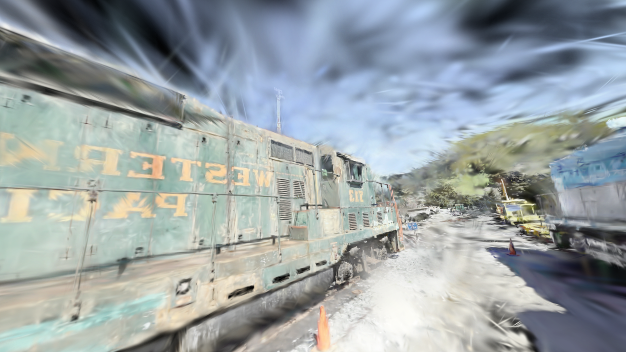
Well, it looks ok, and on my laptop it does suffer a great deal when all the gaussians align. Half a million quads might be too much for him.
Performance analysis
I thought of attempting a more thorough analysis, to compare multiple machines at various resolutions, perhaps using more advanced GPU profiling tooling, but I’ve been cut off from my main desktop PC, and the results on what I have and on the Quest 2 don’t leave much to be asked.
It’s a pretty heavy technique.
On my Matebook D14 from 2018, with a RX Vega 8 I think, I can barely run it: The random gaussians run fine at almost 60FPS at 720, but sorting freezes everything for a couple seconds and the time to render a frame hovers around 200 ms. Expected from such a weak GPU, but highlights how expensive this solution is
On an older ASUS with a 940M (which also needs some heavy dusting) you can already feel the power of an actual GPU, as the scene renders at 25 FPS even when the gaussians are sorted, at 1080p. Lower resolutions raise the performance meaningful.
The Quest 2 is a much sadder story. Likely due to the much higher resolution and difference in GPU architecture, it basically does not run. Unless the scene has only a handful of gaussians, the image tears and breaks up constantly, sorting freezes the entire device and the entire system UI lags as long as LOVR is running in the background. The initial load freezes the entire device for a good 15 seconds.
I also wanted to test it on the desktop with the 1070, expecting it to run fine at 1080 and perhaps acceptably at lowered resolution in VR, but the GPU isn’t feeling too well after the latest move, and I’ll have to diagnose it in the future.
How to use
- Clone the repo from GitHub
- Download LOVR from the official website. Get v17
- Get a gaussian splatting scene, I used the official scenes from the original Paper
- Convert the scene from a binary STL to an ASCII STL
- Install PlyFile
- In Python run
from plyfile import PlyData, PlyElement plydata = PlyData.read('trank_7k_point_cloud.ply') PlyData([plydata.elements[0]], text=True).write('some_ascii.ply') - This will create the ASCII file, in a few minutes
- Move the file to the folder where the code resides
- Call LOVR on the folder and wait!
Other gaussian scenes might work, but the code has some parameters hard coded inside, such as the number of points to render, and the pre-processing might vary in various implementations.
GPU debugging
One big issue with this project was debugging GPU code. Being honest, even writing GPU code was not easy, not just for the technical barriers, but also my lack of good sources.
All the tutorial I found covered only introductory sections and focused mostly on the traditional 3D rendering sections, so Phong lighting and texture mapping, and spent most of the time fighting with C++. Maybe I missed a Holy Grail of tutorials, but I would be confused as where it might be hiding.
Debugging was doubly problematic, as OpenGL does not present any clear logging pathways or tools that resemble things like printf debugging, gdb or similar things. Some solutions exist, but are usually tightly linked with custom engines or libraries, or are hardware specific.
So I made my own:
- The Debug Readback
- The Render Mode Switch
These absolutely unprecedented ideas allowed me to solve quite a few problems.
The Debug Readback is simply an additional Buffer between CPU and GPU, which can be written into by the GPU and is read back at each frame, printed to the console. So a rudimentary logging solutions for numbers. It was a game changer in how it simplified solving some issues and looking at chunks of data, although it still misses any metadata for variables, and requires a lot of thought to use correctly.
The Render Mode Switch is simply using an extra parameter passed to the GPU to switch to different branches of the shader code, allowing me to see debug information in a visual format, using early exit statements to test different sections of code and more. This is still very limited to the fact that values need to be between 0 and 1, but at least some information can be gleamed by the positioning of the colors.
I tried using tools like RenderDoc and an AMD debugging layer, but I could not figure out how to take advantage of them.
And now?
There’s a lot more to explore here. The code is barely working, with ample space to improve and optimize: Using threads to load and run operations, precomputing stuff instead of repeating calculations every frame, reading binary files, using better sorting, identifying GPU optimization, especially VR focused solutions, reading more papers.
But I’ve been working on this for months now, while finishing my Master’s and moving from Austria to Germany, and I want to draw a line for now ad focus on other things.
I hope this was somewhat understandable, if not informative. If you have any suggestions regarding GPU programming resources, GPU debugging and performance testing tools, or anything else please contact me on GitHub, you can also find my email there.