home..

Numerical integration and orbital mechanics

Martino Trapanotto / April 2026 (12677 Words, 71 Minutes)

Motivations and context

Scientific computing was one of my major interests when I decided to study computer engineering, alongside Machine Learning and Computer Vision, but unlike these topics it was not a major part of my curriculum. Harnessing the immense computational power of silicon to probe otherwise intractable problems just seems so cool.
Thus, I decided to explore some aspects of numerical integration for differential equations, and picked the context of Orbital Mechanics, specifically the restricted 2 body problems.
I hoped this would provide a complex enough framework with nonlinear dynamics, while maintaining an analytical solution for reference.

The code for the orbits, the solvers and the data post-processing for the graphs, in Lua and Julia, is available on my GitHub.

Fundamentals of orbital mechanics

Orbital mechanics groups together a wide range of problems that describe the evolution of motion of bodies under gravity.
The general form of the field is highly complex, and spans nonlinear differential systems, general relativity and chaotic systems.
We’ll be considering only a very restricted version of orbital mechanics, the one studied mostly by Kepler and Newton in the 1600s known as the restricted 2 body problem, also known as central force problem.

The general version considers two bodies in motion that interact with each other gravitationally and have comparable masses, like the Earth and the Moon, while the restricted form considers the two bodies to have an extreme difference in mass, and thus one can be considered to be stationary, closer to the Sun and Earth.
This simplified version was developed by Newton in his 1687 Philosophiæ Naturalis Principia Mathematica, to model the evolution of celestial bodies in the solar system, as the western world was slowly moving away from Aristotelian geocentrism towards heliocentrism.

Thus, we consider the central body to be completely static, and we only consider the orbits of the smaller bodies. These bodies do not interact with each other in any other way, only gravity is at play.
If here $\vec{r}$ is the position of the orbiting body and $\mu$ is the gravitational constant of the central body we have the differential equation:

$$\begin{align} \ddot{\vec{r}} = -\left(\frac{\mu}{r^3}\right)\vec{r} \end{align}$$

Describing the relationship between the position $\vec{r}$ and the gravitational force $\ddot{\vec{r}}$, in a second order non linear equation.
This kind of equations are not generally solvable, but Newton’s work proved effective, and he showed that the bodies follow what are called Keplerian Orbits, which are always circles, ellipses, parabolas or hyperboles. They can also be uniquely described by only 6 values, and have a complete analytical form. From Wikipedia

These values can be derived from the State Vector, which consists of the position $\vec{r}$ and speed vector $\vec{v}$:

$$\begin{align*} \vec{h} = \vec{r} \times \vec{v} &\quad \vec{n} = \hat{K} \times \vec{h} \\ \vec{e} = \frac{(v^2 − \frac{\mu}{r} ) \vec{r} −(\vec{r} \cdot \vec{v})\vec{v}}{\mu} &\quad \begin{cases} a = -\frac{\mu}{2E} &\text{if e$\neq$1} \\ a = \infty &\text{if e = 1} \end{cases}\\ i = \arccos(\frac{h_K}{h}) \\ \Omega = \arccos(\frac{n_I}{n}) & \text{, \quad if $n_J$ < 0 then $\Omega=2\pi-\Omega$} \\ \omega = \arccos(\frac{\vec{n}\cdot\vec{e}}{ne}) & \text{, \quad if $e_K$ < 0 then $\omega=2\pi-\omega$} \\ \nu = \arccos(\frac{\vec{e}\cdot\vec{r}}{er}) & \text{, \quad if $\vec{r}\cdot\vec{v}$ < 0 then $\nu=2\pi-\nu$} \\ \end{align*}$$

With these, we can draw and visualize the true reference value for our integrators.
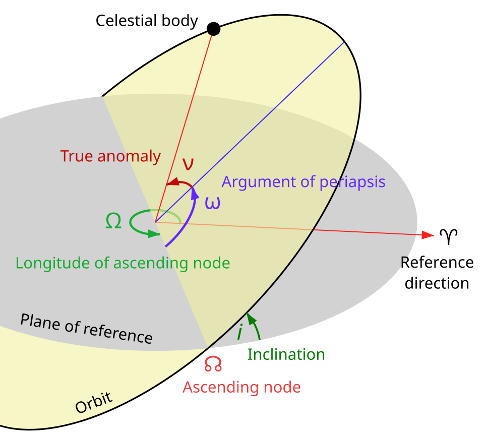
As illustrated in the diagram, $i, \omega$ and $\Omega$ identify the Orbital Plane, where our orbit lays.
Known as True Anomaly, $\nu$ or sometimes $\theta$ is the angle between the periapsis of the orbit and the current position, and is our only time-variant value. The eccentricity $e = |\vec{e}|$ is key, as it differentiates the kind of orbit: the normal elliptical $(e<1)$ orbit of most planets and the parabolic $(e=1)$ or hyperbolic $(e>1)$ which are closer to what comets follow.
We’ll also be able to study the performance of the solvers by analyzing the total energy of the orbit and angular momentum, both of which should be constant in time.

As a fun quirk, in physics and thus orbital mechanics, $I, J , K$ usually indicate respectively $X, Y, Z$, with $Z$ up. Meanwhile LOVR uses Y up.
This introduces some subtle differences in the formulas, and lost me more than a couple weeks, as it requires care in swapping indices and keeping track of all affected values, including vector products like $\vec{n}$ and $\vec{k}$.

The Gonzalrez orbit viewer, this stackexhange on computing orbit parameters from the state vector and the blog orbital-mechanics.space were all instrumental to making this section possible.

Sidenote: True anomaly and time

There’s a very interesting detail in the relationship between time and true anomaly $\nu$, which describes the angle between the body and the periapsis of the orbit, and is the only variable that evolves in time in an orbit.
This relationship has no analytical solution, requiring instead the use of intermediate values and a root finding algorithm.
Let’s see these formulas for elliptical orbits:

$$\begin{align*} &M_e = \frac{2\pi t}{T} = \frac{\mu^2}{h^3} t \left(1 - e^2\right)^{3/2} \\ &M_e = E - e \sin{E}\\ &\tan\frac{E}{2} = \sqrt{\frac{1 - e}{1 + e}}\tan\frac{\nu}{2}\\ \end{align*}$$

Here $t$ is the time since periapsis and $T$ the orbital period, $M_e$ and $E$ are called “Mean anomaly” and “Eccentric anomaly” respectively. For more details on their true geometric meaning, see here.
We can see that going from $\nu$ to $t$ is a set of gnarly formulas, but not a major issue. The reverse problem, computing the 3D position based on time, is much more problematic due to equation $2$.
That’s called a transcendental equation, meaning that at least one side can’t be written as a simple algebraic solution with basic operators.
Thus, there’s no closed finite formula for it, only Taylor series expansions, or using a root finding algorithm.

The most common, and perhaps relevant considering the historical aspect, is the Newton-Raphson method, where we define a function $f(x) = 0$ for which we want to find the zeros, or roots, and staring from a guess $x_0$ we iterate on this advancing towards a better and better approximation: $x_{n+1} = x_n - \frac{f(x_n)}{f'(x_n)}$ In our case, $f(E) = M_e -E + e \sin(E) = 0$, with $f'(E) = 1 - e\cos(E)$, and we can use the previous time step’s $E$ for $x_0$.
With a good initial guess, such as the previous time step’s solutions, this usually converges in only a few steps.

Integration Methods

Now that we have set the stage and context of orbital mechanics, we can try to ignore these beautiful closed solutions and see what we can do with raw computational power instead.
We’ll now introduce the methods used and some known properties of theirs.

We’ll consider first the models in their abstract form, on the general ODE $y'_t=f(t, y_t)$, with $y'_{t_0}, y_{t_0}$ as initial values and $h$ as our time step.
Most of these methods are designed for first order equations, so we’ll also briefly cover their extension to the second order equations of motion.

Euler’s method

Among his immense array of mathematical developments, Euler introduced the first numerical method for differential equations in 1768.

$$y(t+h) = y(t) + hf(t, y(t))$$

A simple and very fast method that simply uses the slope at time $t$ to step linearly.
Thus, for our orbit the formula becomes

$$\begin{align*} &x(t+h) = x(t) + hv(t) \\ &v(t+h) = v(t) + hf(t, x(t), v(t)) \end{align*}$$

This is the first method developed to solve this kind of problems and has limited performance certainties, with an estimated cumulative error of $O(h)$

Euler-Cromer

This method derives very naturally from Euler’s, where we use the new $v(t+h)$ to compute $x(t+h)$, so the final formula is

$$\begin{align*} &v(t+h) = v(t) + hf(t, x(t), v(t))\\ &x(t+h) = x(t) + hv(t+h) \end{align*}$$

This method is a special kind of integrator, called symplectic.
These have unique properties relating to solving equations with certain conditions, and are commonly used in various physical simulation as they’re designed to manage 2nd order equations like those of motion.
We’ll talk about these later.

Runge-Kutta

A much wider family of methods from the early 1900s developed by German mathematicians Carl Runge and Martin Wilhelm Kutta.
These methods combine sequences of smaller perspective step to refine the final step much further, and have become extremely popular methods across engineering, typically the 4th order predictor RK4, thanks to its balance of computational costs and solid error bounds.

A general formulation of the explicit forms of these methods is

$$\begin{align*} &y(t+h) = y(t) + h \sum^s_{i=1} b_i k_i \\ &k_i = f(t+c_i h, y(t) + \sum^i_{j=1}a_j k_j) \end{align*}$$

Here we combine multiple sub-steps $k_i$ with a weighted average in our final estimate.
Each $k_i$ is computed by combining information from their predecessors $k_j$. $a_i$, $b_i$ and $c_i$ are all weights.

These methods are generally favored for their good convergence properties and ease of implementation.
You can see more here:
Runge-Kutta Integrator Overview: All Purpose Numerical Integration of Differential Equations - Steve Brunton
Why Runge-Kutta is SO Much Better Than Euler’s Method - Phanimations

RK2

We consider first the 2nd order version of this, where we use two intermediate evaluations $k_1$ and $k_2$ to better gauge the next integration step.

$$\begin{align*} &k_1 = f(t, y(t)) \\ &k_2 = f(t+\frac{h}{2}, y(t) + \frac{h}{2} k_1) \\ &y(t+h) = y(t) + h k_2 \end{align*}$$

This method should result in $O(h^2)$ global error, a major increment on Euler’s method.

RK4

The 4th order method uses 4 chained estimates to converge closer to the true value.

$$\begin{align*} &k_1 = f(t, y(t)) \\ &k_2 = f(t+\frac{h}{2}, y(t) + \frac{h}{2} k_1) \\ &k_3 = f(t+\frac{h}{2}, y(t) + \frac{h}{2} k_2) \\ &k_4 = f(t+h, y(t) + h k_3) \\ &y(t+/h) = y(t) + \frac{h}{6}(k_1 + 2 k_2+ 2 k_3 + k_4) \end{align*}$$

This is perhaps the most popular multipurpose numerical integrator, used in many off-the-shelf solvers like SciPy’s and MATLAB’s. It has very solid global convergence error of order $O(h^4)$, and thus should be quite stable in the long term.

Jolt

As a final comparison, we use the internal LOVR physics engine, which relies on Jolt.
This is open source game physic engine used in multiple high profile projects like Death Stranding 2 and Horizon: Forbidden West.
The details on how exactly the physics state are pretty complex, but the official docs reference using a Symplectic Euler solver, so something akin to our Euler-Cromer solver.

Results

Considering a 5-minute simulation, we can consider a few data points to compare and contrast our solvers.
Let’s look at absolute error in time first, how do our integrators perform?

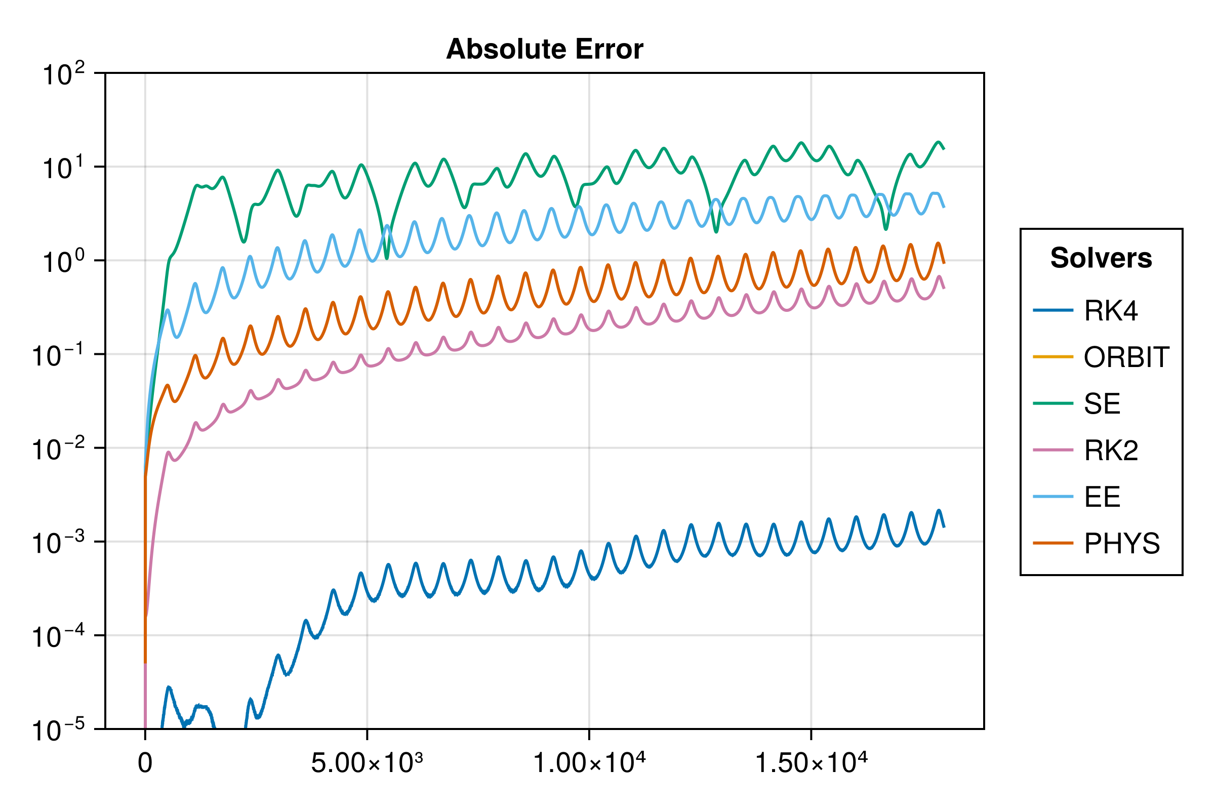
In these diagrams, the ORBIT solver is our analytical solution, so it’ll be generally regarded as the reference value.
In this case, the absolute error is in meters, here on a log10 graph, so small increments are major jumps in error. The ORBIT solver does not appear, as it has 0 error to itself.
It’s easy to observe that the best performers are the Runge Kutta solvers, with the 4th order vastly outperforming all other solvers. The RK2 and Jolt solver perform similarly, with the Extended Euler in a worse position, and the Simple Euler behaving the worst.

But if we look at the graph of total energy of the body, we see a different picture:

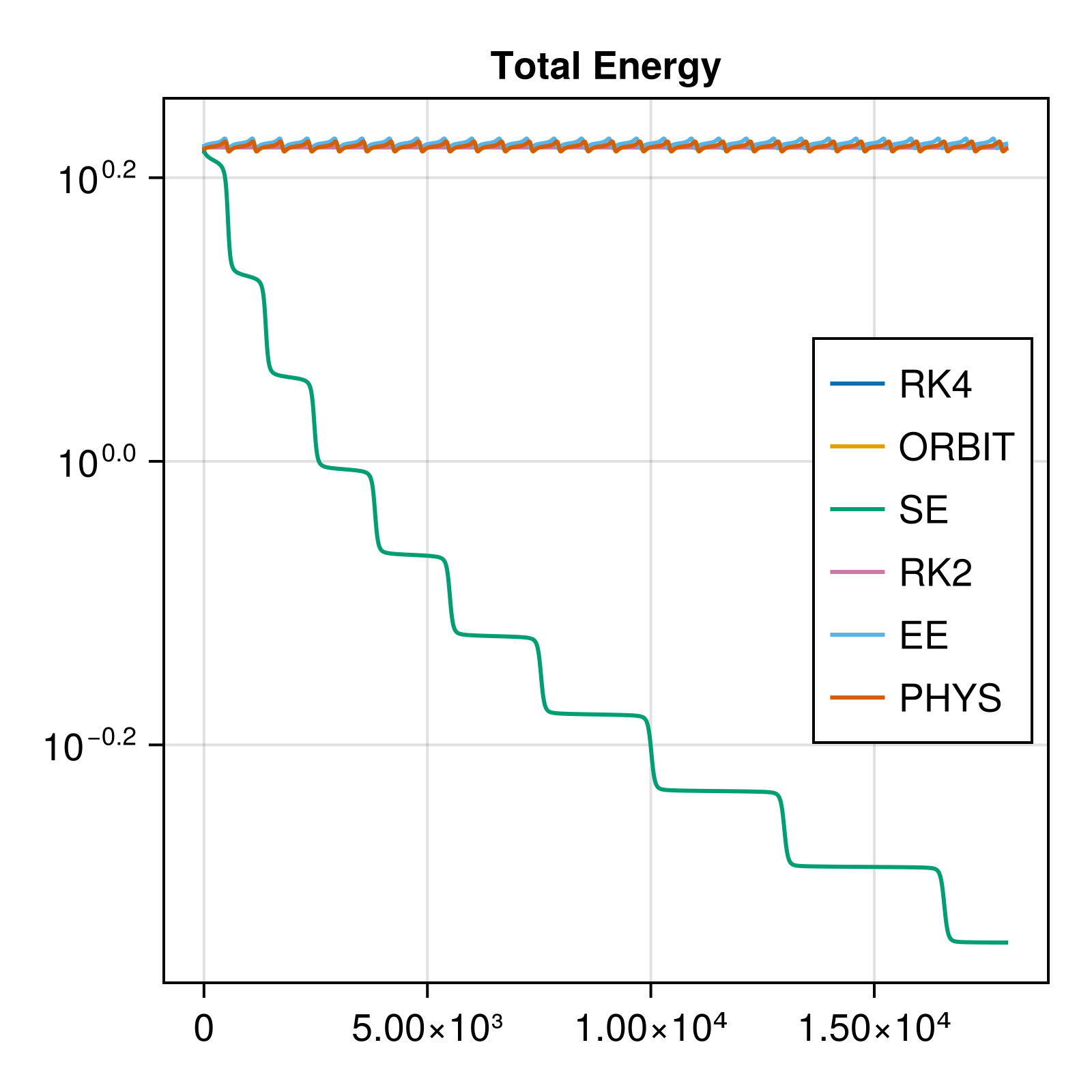
We know that total energy is a conserved property of Keplerian orbits. There’s no external forces, exchange of matter or energy with the outside and no friction, so the conservation is obligatory.
Thus, we observe here that the Simple Euler solver is an outlier in its very poor handling of the orbit’s energy.
These together might indicate to us that RK solvers are our best bet in this context, but the reality is not as simple.

The issue of energy not being conserved is actually shockingly common to various integration schemes: even the high performing RK solvers don’t actually conserve energy or angular momentum in the long term, and will instead tend to drift away on larger timescales.
For many applications this is not an issue, whether because energy conservation is not a factor, or because the task focuses more on precision than maintaining certain physical constraints over long periods.

But we can also notice that the Cromer-Euler integrator also performs remarkably well.
This is no accident, as this solver is actually capable of conserving some properties of the physical system over time very well, and is very important for long term simulations of physical systems such as orbits or plasma fields, where long term stability is more important that exact numerical precision, and where computational costs are impactful.
What’s the key to these solvers’ unique abilities?

Hamiltonian mechanics and symplectic integrators

In 1833, William Rowan Hamilton introduced a novel formulation of mechanics based on the Lagrangian models of 1788. Both of these approaches took a different path from the force-oriented concepts of Newton, and instead defined the world as differential equations.
In contrast to Newtonian mechanics, where all action is defined in terms of forces and vectors, requiring complex geometrical work to solve any problem among other issues, Lagrange and then Hamilton focus directly on the free variables in the equations of the systems. They create novel variables to study the systems, and work on a more abstract notion of action and work, opening the way for more powerful mathematical tools to enter physics.
This leads to different solving approaches, where geometry and forces are in focus, but instead the evolution of the system as a whole by studying these free variables, and describing the behavior of the system through differential equations.
To learn more, watch The origin of Hamiltonian Mechanics - Dr. Jorge S. Diaz and Lagrangian vs Newtonian Mechanics - Abide By Reason.

These new approaches, called analytical mechanics, have been a revolutionary force in physics, paving the way for statistical and quantum mechanics.
While the Hamiltonian is usually described in undergrad physics texts as the sum of kinetic and potential energy $H = U + K$, this is not quite true, and much subtler definitions would be required to fully capture the topic. This is outside the scope of this article, but the curious can read some physics StackExchange posts 1, 2, 3.
For us, the core takeaway is that a Hamiltonian system is defined by having a well-defined function $H$, from which the states of the $2n$ variables $q_i, p_i$ can be defined as $\dot{q_i} = \frac{\partial{H}}{\partial{p_i}}, \dot{p_i} = -\frac{\partial{H}}{\partial{q_i}}$, where $q_i$ usually identifies the free variables of the physical system and $p_i$ the generalized momenta.
For example, in the simple pendulum $q$ is the angle of the pendulum, and $p$ is the associated angular momentum of the system, so given $L$ length and $m$ mass of the pendulum arm:

$$\begin{cases} H = U + K = \frac{p^2}{2mL} - mgL\cos(q) \\ \dot{p} = -\frac{\partial{H}}{\partial{q_i}}= mgL\sin(q) \\ \dot{q} =\frac{\partial{H}}{\partial{p_i}}= \frac{p}{mL^2} \end{cases}$$

This model creates much more compact and flexible tools and methods to describe and work on physical problems, and opens the door to a novel method to represent a system’s state and evolution: Phase Spaces.
These spaces represent the problem not through common 3D coordinates, but solely working with $q_i$ and $p_i$, which capture the complete state of the system in a single $2n$ state vector.
Referring back again to the example of the pendulum, we can see here the pairing of the 2D pendulum and its associated angle and momentum. The path traced in the phase space describes the evolving state of the pendulum only though the angle and the speed.

By Ian Cooper.

Phase space is not only a powerful tool to visualize and comprehend evolving systems, but gives us a new geometrical space to study them from. Here, we can observe convergence and divergence, attractors and repulsors, stability and instability as paths in space, and comprehend their evolution geometrically. See Phase Space: the geometry of Hamiltonian mechanics - Dr. Jorge S. Diaz.
Phase spaces can be used to study systems of any kind, but when we consider most Hamiltonian systems, we can also leverage specific theorems: the most relevant one for our case is Liouville’s Theorem, which identifies that as the Hamiltonian system evolves, areas representing groups of trajectories must be constant in time, see The Code That Revolutionized Orbital Simulation - braintruffle.
In practice, this places a very tight limit to the kind of evolution of the vectors of our system, and will show us why some integrators work so well for these kinds of problems: The space-preserving property has a direct algebraic consequence for any Hamiltonian system, where the transformation matrix that describes the evolution of a system’s state in time must have a Jacobian determinant of 1.
This is a fundamental property of all symplectic systems, and most integration schemes do not maintain this requirement.

We can see this if we consider the example of a body on a spring. The equation of motion in Newtonian terms is $F = \frac{dv}{dt}= -kx$ with $x$ the displacement from the resting position. Given also the simple $v = \frac{dx}{dt}$ we have all the building blocks to try and build our integrators.
Let’s now compute the Jacobian of the Simple Euler and the Euler-Cromer integrators. In a linear system, the determinant of the update matrix that construct the new values given previous values is our Jacobian:

$$\begin{align*} &\text{Simple Euler} \\ x(t+dt) &= x(t) + v(t)*dt \\ v(t+dt) &= -k*x(t)*dt + v(t) \\ \det{J} &= \det\Bigg(\!\!\begin{array}{cc} 1 & dt \\ -k*dt & 1 \end{array}\!\Bigg) \\ &= 1 -k*{dt}^2 \\ \\ &\text{Euler-Cromer} \\ x(t+dt) &= x(t) + v(t+dt)*dt = (1-k*{dt}^2)*x(t) + v(t)*dt \\ v(t+dt) &= -k*x(t)*dt + v(t) \\ \det{J} &= \det\Bigg(\!\!\begin{array}{cc} 1-k*{dt}^2 & dt \\ -k*dt & 1 \\ \end{array}\!\Bigg) \\ &= 1 - k*{dt}^2 + k*{dt}^2 = 1 \\ \end{align*}$$

Here we observe the core issue:
The simple Euler solver’s Jacobian only approximates 1, and only for time intervals $dt$ that tend towards zero.
Inversely, the Euler-Cromer solver has a fixed Jacobian of 1, and thus maintains the geometric structure of the phase space as the system evolves.
This property is of the solver, and extends to non-linear systems, like our orbits, where such a demonstration is not possible, and thus also applies to our orbit problem.
The Runge-Kutta solvers are also generally not symplectic, but have much superior numerical performance, and so work great in our limited case. Real physics simulations very often leverage symplectic solvers instead to ensure longer term stability without requiring increasingly small time steps.

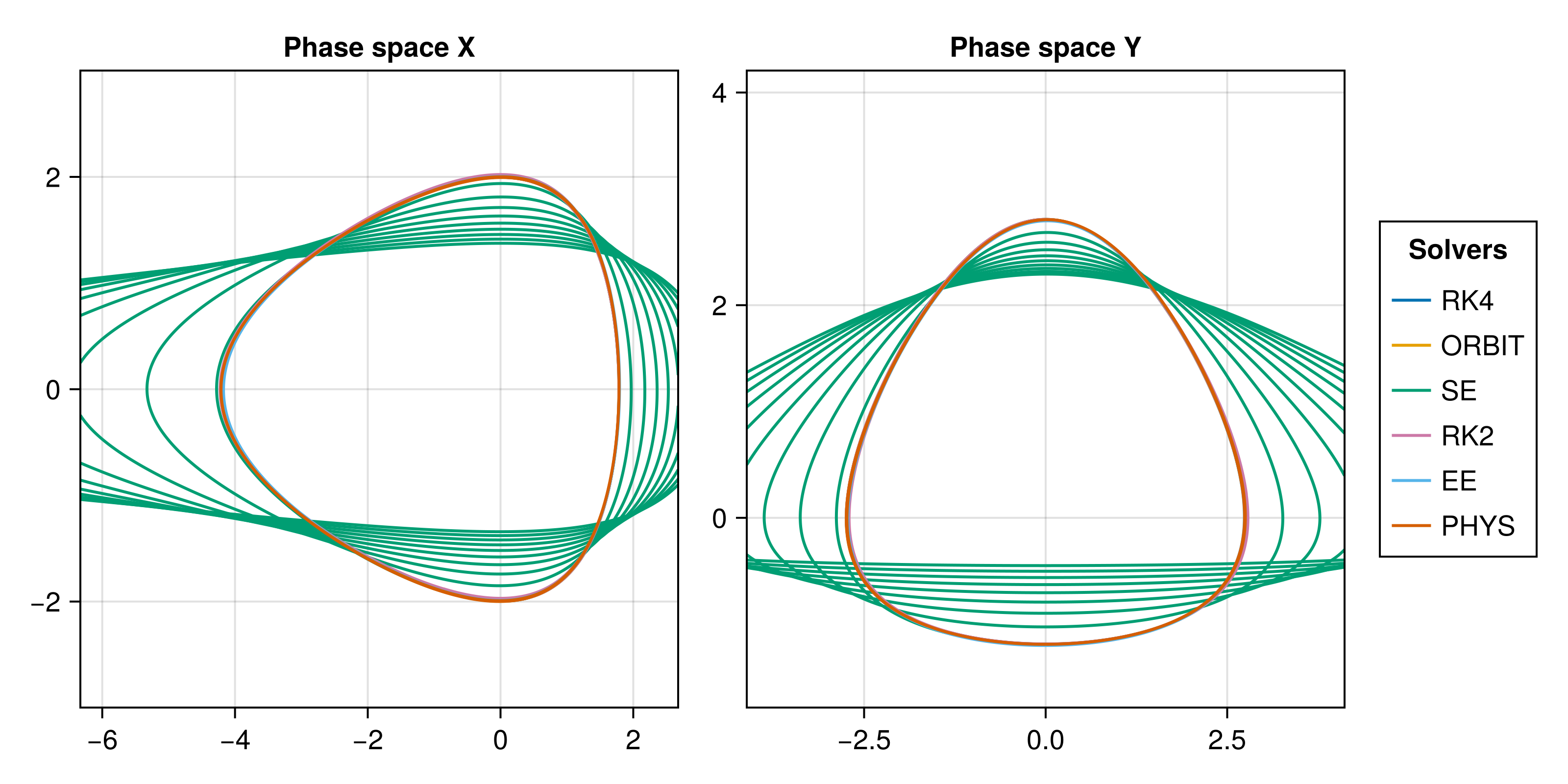
Here we visualize the phase space of the previous orbit, on the perifocal plane.
We can observe the Simple Euler solver diverging from the others in phase space, making it clear how it’s not maintaining the energy and momentum constant, and is deviating from the others.

Conclusions

The clearest conclusion is that common wisdom and industry standard is pretty accurate: Runge Kutta solvers are fast and effective, and the 4th order solver is an amazing tool for all kinds for problems, with only moderate computational costs.

But perhaps more important is how impactful specific knowledge about the problem and the mathematics underlying it are: long term stability does not come from hardware engineering or computer science, but from physics and mathematics.
Especially in the contemporary context of highly optimized solvers and specialized numerical analysis tools, there’s little need for computer scientists to write optimized C algorithms or ASM powered solutions to squeeze as many iterations as possible per silicon atom, at least in the general case.
Embedded systems, computer graphics and high performance environments still need someone to tweak memory usage and find smart workarounds to expensive math functions, but most scientists and engineers just use SciPy or Julia or FORTRAN, harnessing their specialized knowledge instead.

With LLMs, accessing some of these formulas and methods becomes even easier, and perhaps removes some of this from the “necessary reading” pile altogether.
But knowledge is never useless, either in what we discover on the path to it, or in its role as a component of our mental landscape.
Imagine learning a language without the words, only looking at grammar rules, or cooking without knowledge of ingredients and flavors.

No wisdom exists without knowledge.